Fluorescence maturation time - is it a bug or a feature ?
Using fluorescent maturation delays to infer gene expression dynamics from static snapshots of cell-to-cell variability.
Giants this stands onand many more of course!:
M. Elowitz (lab), P. Cluzel (lab), P.-S. Laplace (wiki), and D. Prasher (wiki).
Fluorescence
Fluorescent proteins are an invaluable tool used to visualize cellular processes (Exhibit A: Nobel Prizes 2008, Exhibit B: Nobel Prize 2014, Exhibit C: This mind-blowing video of a brain).
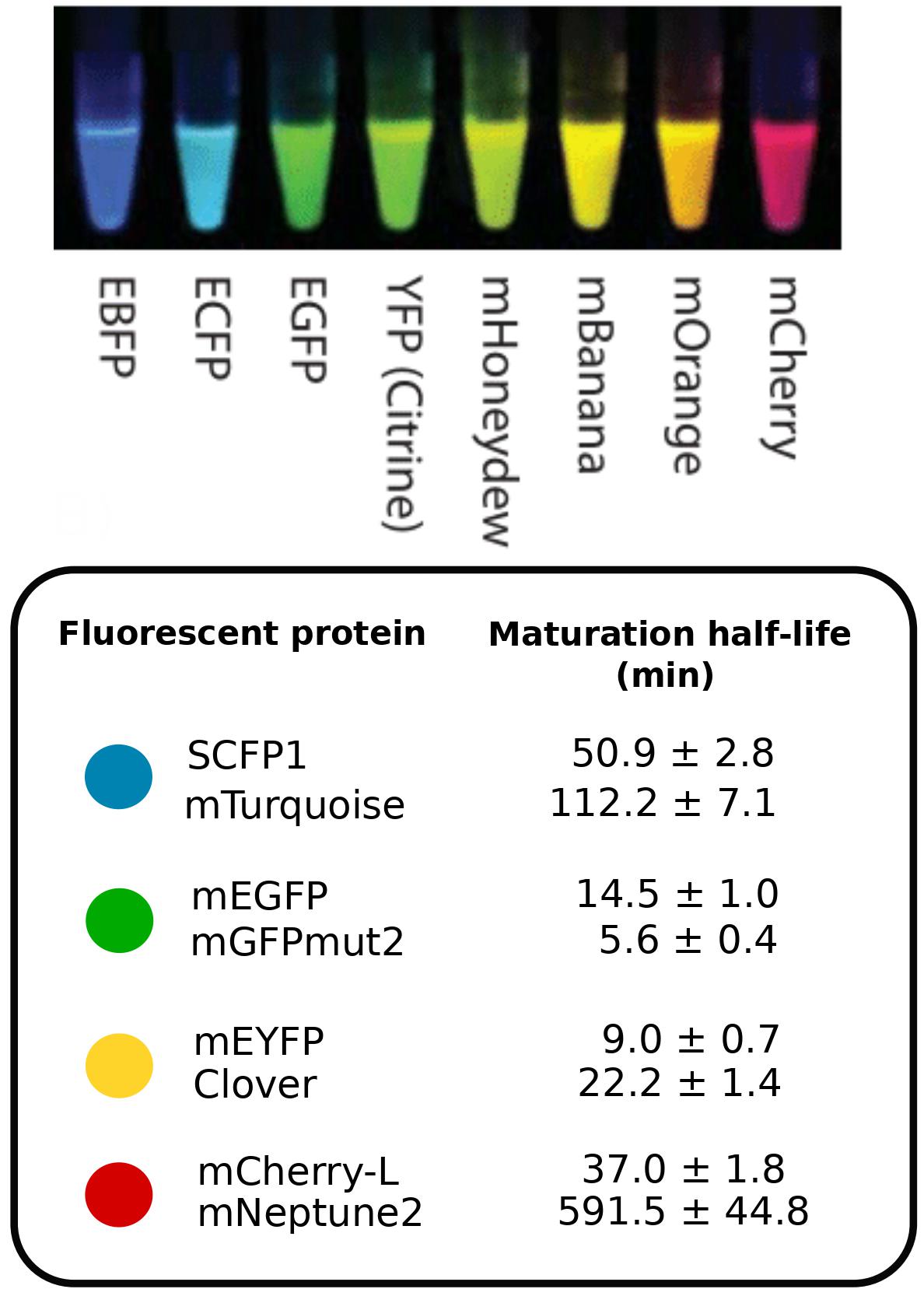
An important caveat when using fluorescent proteins is that freshly produced proteins are dark and take time before they fluoresce. The time that a fluorescent protein takes to become fluorescent is called the maturation time, and it can range from minutes to hoursThis is a fascinating and complex process in itself. Fluorescent proteins with short maturation times are thus used to avoid delays when probing dynamic systemsThe figure on the right is taken from this great [post](http://book.bionumbers.org/what-is-the-maturation-time-for-fluorescent-proteins/) on fluorescent maturation times..
Fluorescent maturation delays are analogous to the delayed response of COVID-19 case numbers. Delays in the onset of symptoms, the analyzing of tests, and the reporting of cases lead to a non-instantaneous read-out of the actual number of infections. Such delays are obviously bad for following (or controllingSee COVID-19 pandemic) dynamics in real-time, but there is an additional effect: the delays in the individual reports of infection are random and not a fixed number, which causes the average variability of the overal signal to be affected. For example, even if COVID-19 case numbers were delayed by a year, but the delay is always exactly the same, we could still recover the maximum number of cases that actually occurred from retrospective time-traces. However, if some of the cases get reported immediately, some take months, and some take a year, the whole dynamics are washed out, and we can no longer identify the size of the peak. The variability of the curve will be washed out due to the probabilistic delay of individual reports. Similarly, the same is true for fluorescence levels in cells because the maturation time of an individual protein is randomMost are exponentially distributed, although some look more like a double exponential. The key is that it is not a fixed delay, i.e., if a fluorescent protein has a 20 min maturation time, some will take 1 min and some will take 40 min to mature. and not a fixed number. Picking a fluorescent protein with fast maturation is thus a key experimental considerationOther properties like brightness and toxicity matter as well., as large maturation times lead to this time-averaging effect in the fluorescence levels, acting as an experimental bug that washes out the information in the observed signal.
Bug or Feature?
However, instead of focusing on minimizing this experimental bug, we asked: can we use this built-in time-averaging effect of fluorescence levels to our advantage? The answer is yes we can!TM This is because the degree to which an exponentially distributed delay washes out a signal depends on the dynamics of the signal itself. As a result, the variability of a time-averaged signal implicitly encodes information about the dynamics of the upstream signal It turns out that the variability of a time-averaged signal corresponds to the Laplace transform of the upstream signal..
In particular, if we have two different fluorescent proteins X and Y reporting the same upstream signal, i.e., the transcription rate of a gene of interest, then the differences in variability will tell us something about the time-scale of the transcription rate variability. In fact, it’s not just the time-scale of the invisible upstream dynamics of the signal that matters, but also its temporal structure! That’s the entire (very simple) idea we are exploiting. The rest is just filling in the mathematical details which are all in our paperSomewhere in Appendix A, Appendix B, Appendix C, Appendix D, Appendix E, Appendix F, Appendix G, Appendix H, Appendix I, Appendix J, Appendix K, Appendix L. Yes, we had to use almost the whole alphabet..
Time-lapse microscopy data of single cells expressing two fluorescent proteins that share an oscillating transcription rate This is work in progress. The fluorescent proteins were engineered to report the activity of a synthetic oscillator known as the Repressilator..
For example, oscillations are different from stochastic signals. Time-averaged responses of the latter are constrained by
\[T_{m} \leq \frac{CV_{x}}{CV_{y}}\]
where \(\tau_{mat,y}/\tau_{mat,x}\) is the ratio of maturation timesMaturation times have recently been precisely measured thanks to amazing from the Cluzel lab, with all their data publicly available. of the two fluorescent proteins, and CV is the coefficient of variation obtainable from static snapshots of cell-to-cell variability. Any violation of this inequalityWe derive constraints on whole classes of systems so as to make few assumptions that can be tested. Here our classes are defined by co-regulation and exponential maturation kinetics. implies that the transcription must be oscillating, even without having to follow cells over time or directly observing the transcription rate. This is crucial, because in recent years there has been an explosion of data produced from high-throughput methods like single-cell RNA sequencing and flow cytometry. These methods lack temporal resolution and produce static snapshots of cell-to-cell variability. A key aim of systems biology is to translate such static datasets into gene expression dynamics.
Engineering co-regulated fluorescent reporters to readout a signal of interest is not new. In fact, such “dual reporters” have previously been used to quantify sources of non-genetic variability in gene expressionCredit for this brilliant idea goes to Michael Elowitz who first used identical co-regulated reporters just like "identical twins" to quantify sources of variability in previous work. However, a fundamental issue remains when interpreting cell-to-cell variability: we generally do not know whether a component’s variability is due to stochastic upstream noise or whether a component is driven by deterministic variability. The above equation can thus become and experimental tool to distinguish cell-to-cell variability that is caused by deterministic oscillationsThere are no truly deterministic oscillations in cells. Every signal will be to some extent stochastic, but we can still define signals as oscillatory if their stochasticity is not so strong as to wash out the periodicity of an oscillatory signal. from variability due to stochastic fluctuations.
Future work
There are quite a few more ideas in this paper (such as detecting feedback), and if you’re interested you can read about them here. Currently we are working on an experimental collaboration to test these results in live cells using a synthetic biology approach. We hope to share with you the results of these experiments another time.
 Fluorescent proteins are an invaluable tool used to visualize cellular processes (Exhibit A: Nobel Prizes 2008, Exhibit B: Nobel Prize 2014, Exhibit C: This mind-blowing video of a brain).
An important caveat when using fluorescent proteins is that freshly produced proteins are dark and take time before they fluoresce. The time that a fluorescent protein takes to become fluorescent is called the maturation time, and it can range from minutes to hours
Fluorescent proteins are an invaluable tool used to visualize cellular processes (Exhibit A: Nobel Prizes 2008, Exhibit B: Nobel Prize 2014, Exhibit C: This mind-blowing video of a brain).
An important caveat when using fluorescent proteins is that freshly produced proteins are dark and take time before they fluoresce. The time that a fluorescent protein takes to become fluorescent is called the maturation time, and it can range from minutes to hours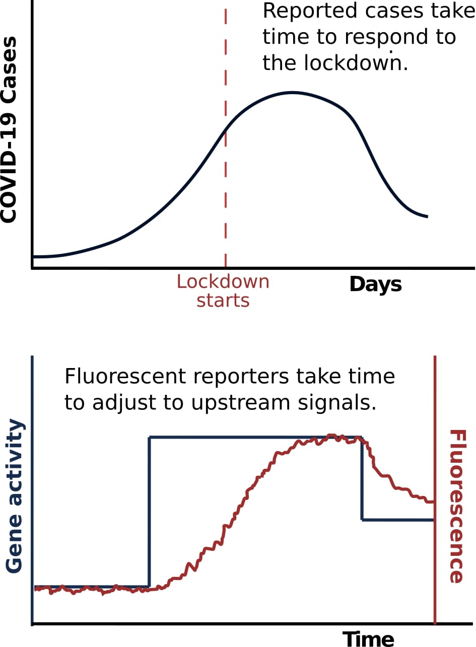 For example, even if COVID-19 case numbers were delayed by a year, but the delay is always exactly the same, we could still recover the maximum number of cases that actually occurred from retrospective time-traces. However, if some of the cases get reported immediately, some take months, and some take a year, the whole dynamics are washed out, and we can no longer identify the size of the peak. The variability of the curve will be washed out due to the probabilistic delay of individual reports. Similarly, the same is true for fluorescence levels in cells because the maturation time of an individual protein is random
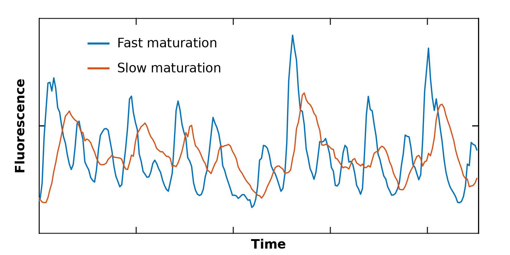
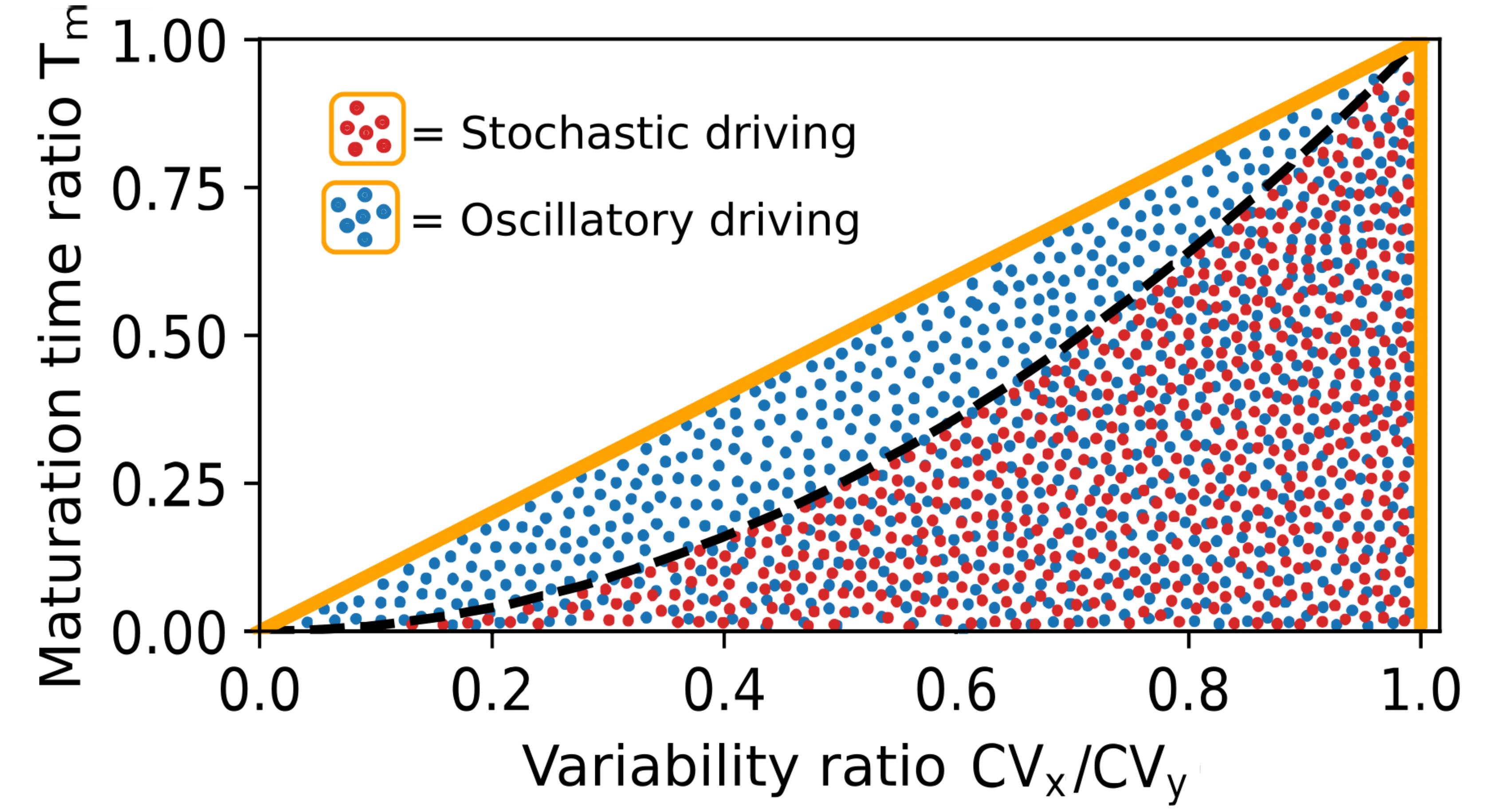 where \(\tau_{mat,y}/\tau_{mat,x}\) is the ratio of maturation times
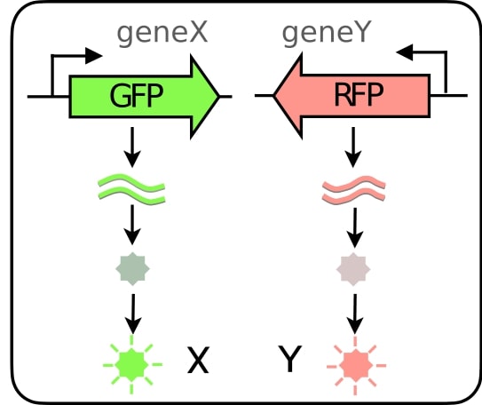 Engineering co-regulated fluorescent reporters to readout a signal of interest is not new. In fact, such “dual reporters” have previously been used to quantify sources of non-genetic variability in gene expression